Google just published a set of papers that could change how much memory AI models need to think. The technique is called TurboQuant, and it compresses a critical part of how large language models work by 5-6x, with essentially zero loss in quality. If you’ve ever wondered why running AI locally requires a beastly GPU, or why API providers charge per token, this is directly relevant.
Here’s the short version: TurboQuant makes AI models smaller at runtime without making them dumber.
The Memory Problem Nobody Talks About
When a large language model generates text, it doesn’t just read your prompt and spit out an answer. It maintains a running memory called the key-value (KV) cache. Think of it like a notepad the model keeps while writing. Every token it has processed gets a key (what is this?) and a value (what does it mean?), and the model refers back to this notepad constantly to decide what to write next.
The problem: this notepad gets huge. For a model processing a long document or conversation, the KV cache can consume more memory than the model weights themselves. A 8-billion parameter model might need 16 GB for its weights, but another 10-20 GB just for the KV cache when processing a long context window.
This is why longer conversations cost more. It’s why running models with 1 million token contexts requires server-grade hardware. And it’s why your MacBook can run a small model but chokes on anything ambitious.
What TurboQuant Actually Does
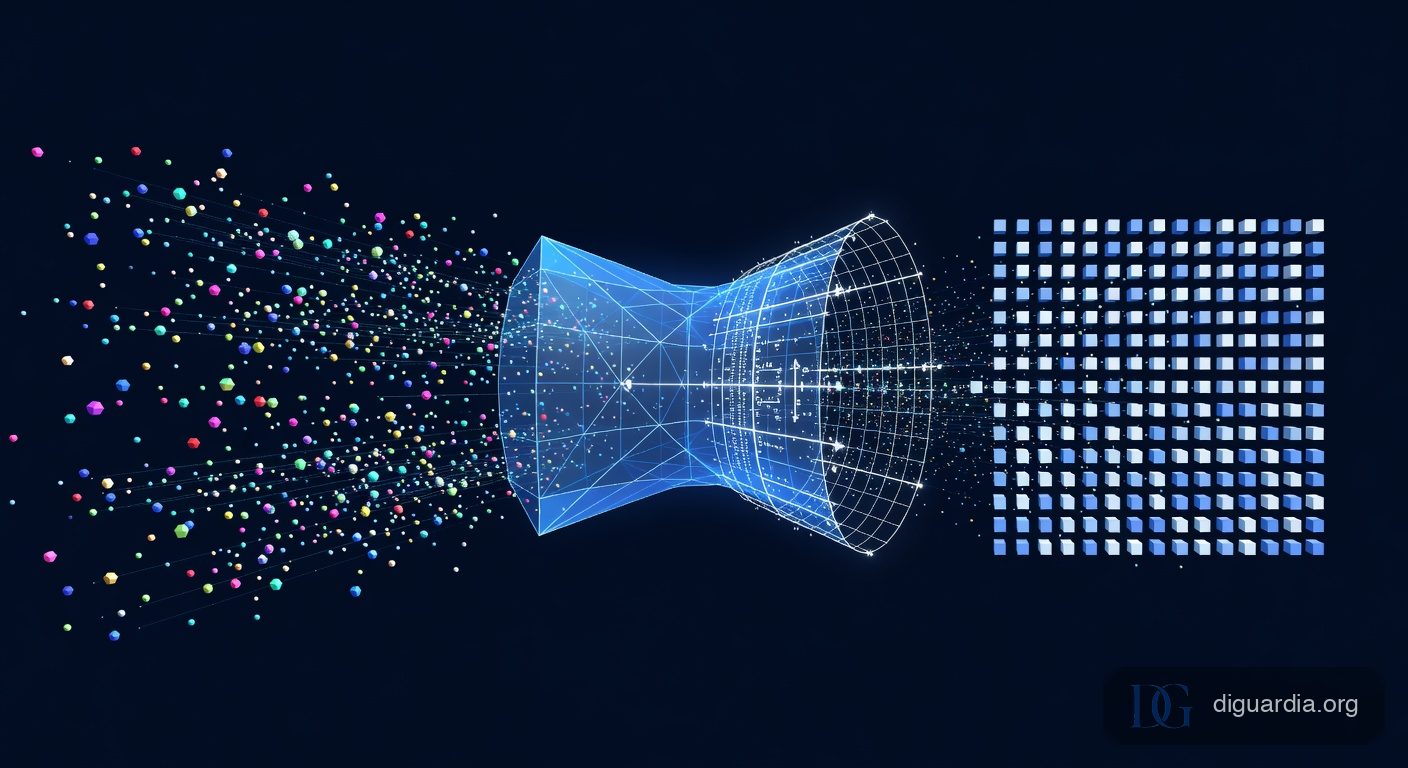
TurboQuant compresses the KV cache from 16-bit numbers down to just 3-4 bits per value. That’s a 4-5x reduction in memory. The clever part is how it does it without losing accuracy.
Traditional compression (quantization) works by rounding numbers. Take a 16-bit float, round it to fit in 4 bits, accept some error. The problem is that real model data isn’t evenly distributed. Some values are huge outliers, and those outliers force you to spread your limited bits across a wide range, wasting precision on the common values.
TurboQuant’s trick is a random rotation. Before quantizing, it multiplies all vectors by a fixed random matrix. This sounds counterintuitive, but there’s solid math behind it. The Central Limit Theorem tells us that when you mix many random values together, the result converges to a predictable bell curve. After rotation, the data follows a known distribution regardless of what the original data looked like.
Once you know the distribution in advance, you can design the perfect compression grid for it. No need to analyze the data, no need to store extra calibration parameters. One precomputed grid works for everything.
The full process has three steps:
- Normalize and rotate. Store the vector’s length as a single number, then apply a shared random rotation matrix. Every vector gets the same rotation, so the decoder can trivially reverse it.
- Snap to a precomputed grid. Each coordinate gets rounded to the nearest point on a grid that’s been optimized for the known post-rotation distribution. At 3 bits, that’s 8 possible values per coordinate. This is the only lossy step.
- Fix the bias with a 1-bit residual. The rounding introduces a small systematic error in dot products (attention scores). TurboQuant applies a technique called Quantized Johnson-Lindenstrauss (QJL) to encode the residual error in just 1 extra bit, making the dot product estimates unbiased.
The result: at 3.5 bits per channel, TurboQuant achieves “absolute quality neutrality” on standard benchmarks. The compressed model produces the same outputs as the uncompressed one. At 2.5 bits, there’s marginal degradation. The paper also reports up to 8x speedup in computing attention on H100 GPUs, because smaller data means less memory bandwidth consumed.
Why This Matters Beyond the Math
The practical implications ripple out in several directions:
Longer context windows get cheaper. The KV cache is what makes long contexts expensive. Compress it by 5x and a 1 million token context suddenly requires the memory of what 200K tokens used to need. One HN commenter estimated this could effectively turn a 1M context system into a 4M context system on the same hardware.
Local inference gets more feasible. If you’re running models on your own hardware (a laptop, a gaming PC, a Mac Studio), the KV cache is often the binding constraint for context length. Shrinking it means you can have longer conversations or process larger documents before hitting memory limits.
API costs could drop. For companies like Google serving billions of queries, every byte of GPU memory per request translates to real infrastructure cost. A 5x reduction in KV cache memory means more concurrent users per GPU, which eventually flows through to pricing.
Vector search gets faster too. TurboQuant isn’t just for LLMs. The same technique applies to vector databases used in search and retrieval-augmented generation (RAG). The paper shows superior recall compared to product quantization baselines, with near-zero indexing time. If you’re building applications that search through embeddings, this is worth watching.
How It Compares to Other Approaches
TurboQuant targets the KV cache specifically. It’s worth understanding where it sits relative to other compression techniques:
- Weight quantization (GPTQ, AWQ, etc.) compresses the model’s parameters. TurboQuant doesn’t touch weights. These are complementary; you can use both.
- Multi-Head Latent Attention (MLA), popularized by DeepSeek, redesigns the attention mechanism to produce smaller KV entries during training. It’s more invasive (must be baked in from the start) but targets the same bottleneck. TurboQuant can be applied post-training, and the two could be combined.
- KIVI, a prior KV cache quantization method, is the main baseline TurboQuant beats. The key difference is that KIVI (and similar methods) need to store calibration constants per data block, adding 1-2 bits of overhead that partially defeats the compression. TurboQuant’s rotation trick eliminates this overhead entirely.
What the Developer Community Thinks
The Hacker News discussion (500+ points, 146 comments) revealed a mix of excitement and skepticism. Some highlights:
Implementation is already happening. Within a day of the blog post, someone had an implementation in llama.cpp, and a group published an independent PyTorch implementation claiming “99.5% attention fidelity.” The llama.cpp implementation is reportedly tiny in terms of lines of code, with one commenter noting they “could see an implementation being merged in 4-6 weeks.” Apple’s MLX team also confirmed the accuracy results.
The blog post itself caught flak. Multiple commenters called Google’s explanation poorly written, with one saying it was “the worst lay-people explanation of an AI component I have seen in a long time.” The animated visualization for PolarQuant was called “straight up nonsensical.” Several people suspected the blog post was AI-generated, pointing to phrases like “this clever step” and “redefining efficiency” as tells. The gap between the quality of the actual research and the quality of its communication was a recurring theme.
A prior art dispute surfaced. A researcher pointed out that the core technique of applying geometric rotation before quantization for bias correction was introduced in a 2021 NeurIPS paper called DRIVE, and that they’d presented the work in a private talk at Google. They weren’t claiming theft, but noted the overlap should be acknowledged in the paper. Another commenter replied: “This is a classical technique, Johnson-Lindenstrauss etc. Rediscovered every few months.”
GPU efficiency was questioned. Some commenters noted that while the paper reports accuracy-vs-space results, the end-to-end latency claims (up to 8x speedup) haven’t been independently reproduced. One commenter wrote: “Polar coordinates are absolute poison for parallel GPU compute.” Though another pointed out the actual implementation uses Cartesian grid centroids, not polar coordinates at runtime.
A particularly detailed explanation from user photon_lines became the thread’s most upvoted comment, walking through the math step by step using the analogy of data bins and rounding. Worth reading if you want to go deeper.
The Bigger Picture
AI efficiency research has been quietly compounding. Building a GPT from scratch today takes a fraction of the compute it did two years ago. Inference costs have dropped 100x since GPT-3. TurboQuant represents another step in this trend, but it’s a meaningful one because it targets a bottleneck (the KV cache) that becomes proportionally more expensive as context windows grow.
The paper was submitted in April 2025 and will be presented at ICLR 2026. It’s likely already deployed in Google’s Gemini models. The fact that independent implementations appeared within 24 hours of the blog post, and that the core algorithm is small enough to fit in a short pull request, suggests this will spread quickly through the open-source ecosystem.
For developers building with LLMs, the takeaway is straightforward: the memory wall for long-context inference is getting pushed back. Models that needed enterprise GPUs for 100K+ contexts will eventually run with the same quality on consumer hardware. That’s not hype; it’s compression math catching up to the problem.
The three papers behind TurboQuant are:
- TurboQuant: Online Vector Quantization with Near-optimal Distortion Rate (ICLR 2026)
- PolarQuant: Quantizing KV Caches with Polar Transformation (AISTATS 2026)
- Quantized Johnson-Lindenstrauss (QJL) (AAAI 2025)
If you want to see the algorithm visually, this interactive animation lets you step through every stage: normalize, rotate, quantize, reconstruct. Add your own points and watch the compression error change as you adjust the bit depth.